BSA analysis exercise instructions for BioHPC Lab

Contact

Questions related to this exercise should be directed to Cheng Zou (cz355@cornell.edu) and Qi Sun (qisun@cornell.edu).

Data used in the exercise

Soyk, S., Lemmon, Z.H., Oved, M., Fisher, J., Liberatore, K.L., Park, S.J., Goren, A., Jiang, K., Ramos, A., van der Knaap, E. and Van Eck, J., 2017. Bypassing negative epistasis on yield in tomato imposed by a domestication gene. Cell, 169(6), pp.1142-1155.

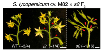
To map j2 and ej2 simultaneously, they performed genome sequencing on pools of DNA from s2, j2, and WT F2 segregating plants.

1.Log in to your workshop machine

The machine allocations are listed on the workshop website: https://biohpc.cornell.edu/ww/machines.aspx?i=112. Details of the login procedure using ssh or VNC clients are available in the document https://biohpc.cornell.edu/lab/doc/Remote_access.pdf. Use your ssh client with BioHPC Lab credentials to open an ssh session. If you wish, you can open multiple sessions to have access to multiple terminal windows (useful for program monitoring). Alternatively, use the VNC client to open a VNC graphical session (you will need to first start the VNC server on the machine from “My Reservations” page reachable from https://biohpc.cornell.edu after logging in to the website. To close the VNC connection, click on the “X” in top-right corner of the VNC window (but DO NOT log out!). This will ensure that your session (all windows, programs, etc.) will keep running so that you can come back to it by logging in again.

2. Prepare the working directory and download sequence files.

1. Connect to your assigned computer. If you do not know how, follow the instruction at http://cbsu.tc.cornell.edu/lab/doc/Remote_access.pdf (Read the section under “Connection by ssh”. There are separate instructions for Windows and Mac users)

cd /workdir
mkdir <yourID>
cd <yourID>

2. Copy the exercise files from the shared location to your scratch directory (it is essential that all calculations take place here):

cp -r /shared_data/BSA_workshop_2018/* ./

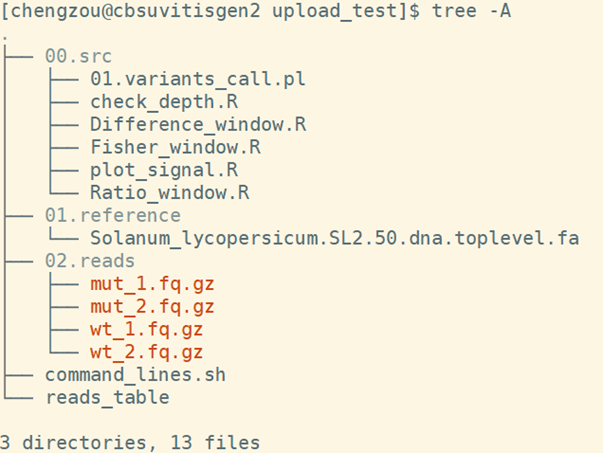
When the copy operation completes, verify by listing the content of the current directory with the command ls -al. You should see 3 folders: one for all the scripts, one for the reference and one for four read files. The command_lines.sh contains all the commands that in this pipeline. Reads_table is a txt file that includes the sample information. It will be introduced in detail in part4.

3. Prepare reads (from public database)

Do not run this codes. The raw data have been downloaded. The command enclosed here is just for your reference. To speed up the calculations, the data has been down-sampled using reads that were mapped to chr3 only. If you are interested in testing the entire data, you can download it from NCBI.

fastq-dump --split-files --gzip  SRR5274882
fastq-dump --split-files --gzip  SRR5274880
wget ftp://ftp.ensemblgenomes.org/pub/plants/release-35/fasta/solanum_lycopersicum/dna/Solanum_lycopersicum.SL2.50.dna.toplevel.fa.gz

4. Build genome index

After it completes, list the content of subdirectory genome. The files reference.fasta.fai and reference.fasta.dict are simple text files summarizing chromosome sizes and starting byte positions in the original FASTA file. The other files constitute the BWA index

### rename the file to simplify the name
cd 01.reference
ln -s Solanum_lycopersicum.SL2.50.dna.toplevel.fa reference.fasta

bwa index reference.fasta 
java -jar /programs/picard-tools-2.9.0/picard.jar CreateSequenceDictionary R=reference.fasta 
samtools faidx reference.fasta 

cd ..

5. Reads mapping and variance calling

A integrated pipeline has been developed. It includes reads mapping, alignment sorting and index, mark duplicated reads, variance calling and filtering. The final result includes the

perl 00.src/01.variants_call.pl reads_table 03.bam/ 01.reference/reference.fasta

reads_table : A three column tab delimited txt file file, which contains the sample name, the 5 end reads location , the 3 end reads location.

03.bam: The directory for the output. The output directory can not be an exist directory.

01.reference/reference.fasta: the location of the reference file.

In the log file, 03.bam/bwalog contain all commands that this script execute.

Step 1: Align the reads, sort and index the results:

bwa mem -t 8  -M -R '@RG\tID:mut\tSM:mut' 01.reference/reference.fasta 03.bam /fixed6.mut_1.fq.gz 04.bam/fixed6.mut_2.fq.gz  | samtools sort -@ 8 -o 03.bam /mut.sorted.bam -  2>> 03.bam/bwalog
java -jar /programs/picard-tools-2.9.0/picard.jar BuildBamIndex INPUT= 03.bam /mut.sorted.redup.bam QUIET=true VERBOSITY=ERROR

bwa mem -t 8  -M -R '@RG\tID:wt\tSM:wt' 01.reference/reference.fasta 03.bam/ fixed.wt_1.fq.gz 04.bam/fixed.wt_2.fq.gz  | samtools sort -@ 8 -o 03.bam/wt.sorted.bam -  2>> 03.bam//bwalog
java -jar /programs/picard-tools-2.9.0/picard.jar BuildBamIndex INPUT=04.10bam//wt.sorted.redup.bam QUIET=true VERBOSITY=ERROR

-M : mark shorter split hits as secondary (for Picard compatibility).

Step 2: Filtering the alignments, mpileup and variance calling

samtools  mpileup -t AD,DP -C 50 -Q 20 -q 40 -f 01.reference/reference.fasta   03.bam/mut.sorted.bam  03.bam/wt.sorted.bam  -v  | bcftools call --consensus-caller --variants-only --pval-threshold 1.0 -O z  -o  03.bam/Out.vcf.gz

-t, --output-tags LIST optional tags to output:

DP,AD,ADF,ADR,SP,INFO/AD,INFO/ADF,INFO/ADR []

-g, --BCF generate genotype likelihoods in BCF format

-v, --VCF generate genotype likelihoods in VCF format

-C, --adjust-MQ INT adjust mapping quality; recommended:50, (unique hit of the reads)

-Q, --min-BQ INT skip bases with baseQ/BAQ smaller than INT [13]

-q, --min-MQ INT skip alignments with mapQ smaller than INT [0]

-f, --fasta-ref FILE faidx indexed reference sequence file

Step 3: Filtering the variances

bcftools filter  -g10  -G10 -i '(DP4[0]+DP4[1])>1 & (DP4[2]+DP4[3])>1 & FORMAT/DP[]>5'  03.bam/Out.vcf.gz  |    bcftools view -m2 -M2  -  -O z -o 03.bam/filter.vcf.gz

-g, --SnpGap filter SNPs within base pairs of an indel

-G, --IndelGap filter clusters of indels separated by or fewer base pairs allowing only one to pass

-i : expression of Variance that will be included:

(DP4[0]+DP4[1])>1 & (DP4[2]+DP4[3])>1 Both reference allele and alternative allele must be support by at least 2 reads.

FORMAT/DP[]>5 for each sample, there must be more than five reads

Step 4: Extract information for downstream analysis

bcftools  query   -i 'TYPE="SNP"'  -f '%CHROM\t%POS\t%REF\t%ALT{0}\t%DP[\t%AD]\n' 03.bam/filter.vcf.gz | sed 's/[,]/\t/g' - >03.bam/filter.vcf.txt

Results of the run

*.sorted.bam and bai : Sorted and index bam file

Out.vcf.gz: raw variance calling in vcf format

filter.vcf.gz: filtered variances in vcf format

filter.vcf.txt: filtered variances in txt format

Optional Check distribution of the depth in each pool

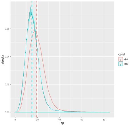
R --vanilla --slave --args  filter.vcf.txt  < ../00.src/check_depth.R

The summary statistics of the total depth will be calculated. The result includes a screen printing summary and a density plot.

6. Statistics calculation

For each method, the statistics are first calculated for each site. And then the median statistics were summarized for each window. Two library were used in the script, one is "dplyr", the other is "CMplot"

Method1: △SNP index

R --vanilla --slave --args  filter.vcf.txt  < ../00.src/Difference_window.R 
R --vanilla --slave --args  filter.vcf.txt.abs_diff_window.txt   < ../00.src/plot_signal.R 

Method 2: ratio of allele frequency

R --vanilla --slave --args  filter.vcf.txt  < ../00.src/Ratio_window.R 
R --vanilla --slave --args  filter.vcf.txt.ratio_window.txt   < ../00.src/plot_signal.R 

Method 3: fishier exact test

R --vanilla --slave --args  filter.vcf.txt  < ../00.src/Fisher_window.R 
R --vanilla --slave --args  filter.vcf.txt.fisher_window.txt  < ../00.src/plot_signal.R 

A few notes of the R script

• Window size in the script is 1 Mbp, steps is 100 kpb

• Only considering contigs >1 Mbp

• Chr name can be any characters, with or without “chr”

• You can manually modify the result ( filter.vcf.txt.abs_diff_window.txt ) to get rid of undesired scaffolds or contigs.