Orthology and Phylogeny

1. Prepare software and data files

1.1 Install the software "figtree" on your laptop.

Go to the web site: https://github.com/rambaut/figtree/releases . Download the software file based on your system.

Windows users can download the file: FigTree.v1.4.4.zip, de-compress. To run the software, double click the file "figtree.jar" located inside the lib directory. (Double click "figtree.exe" might not work for some computers)

Mac users can download the file FigTree.v1.4.4.dmg. Double click to install.

1.2 Prepare the working directory on the Linux server.

The "cp -r" command would copy the whole directory of project3.

mkdir /workdir/$USER
cp -r /shared_data/alignment2020/project3 /workdir/$USER/
cd /workdir/$USER/project3

2. Construct the phylogeny using RAxML-ng

In this exercise, you will use RAxML-ng to build phylogenetic trees from two Multiple Sequence Alignment (MSA) files. "prim.phy" is a PHYLIP formatted file of a primate gene (DNA sequences). "leafy_align.fas" is a FASTA formatted file of a plant gene (protein sequences).

The raxml-ng is a tool with several different functions (Tutorial: https://www.preprints.org/manuscript/201905.0056/v1 ). We will use five of them in this exercise: "check", "search", "bootstrap", "evaluate" and "support". To run the "check" function, for example, you need to use the command "raxml-ng --check". Run "raxml-ng" without function name defaults to the "search" function.

2.1 Verify the format and data consistency of the input files

RAxML-NG can read MSA files in FASTA, PHYLIP and CATG formats. The "check" function automatically detect and verify the file formats.

## add raxml-ng to the PATH
export PATH=/programs/raxml-ng_v1.0.1:$PATH

### verify the prim.phy file with DNA sequences
raxml-ng --check --msa prim.phy --model GTR+G 

### verify the leafy_align.fas file with protein sequences
raxml-ng --check --msa leafy_align.fas --model LG+G4

If you see the message "Alignment can be successfully read by RAxML-NG", your input files are ok.

2.2 Inferring ML trees

Run "raxml-ng search" and find the best ML tree.

• Here you will use the GTR_GAMMA model for DNA sequences ("--model GTR+G") ;
• "--msa": input MSA file;
• "--prefix": prefix of output file names;
• By default, it would perform 20 tree searches using 10 random and 10 parsimony-based starting trees. While it is a reasonable choice for most practical cases, given enough computing resources, you might want to increase the number of starting trees to explore the tree space more thoroughly, e.g. with the parameter " --tree pars{25},rand{25} ". On the other hand, you can do "raxml-ng --search1" to perform a quick-and-dirty search from a single starting tree.

raxml-ng --threads 2 --msa prim.phy --model GTR+G --prefix A1

Out of the 20 trees, the best tree is saved to a file "A1.raxml.bestTree".

There is a log file named "A1.raxml.log", with likelihoods of all 20 trees. Use "grep" to extract the 20 "logLikelihood" values.

grep "logLikelihood:" A1.raxml.log
grep "Final" A1.raxml.log

You should see output like:

[00:00:02] [worker #1] ML tree search #2, logLikelihood: -5708.924752 [00:00:02] [worker #0] ML tree search #1, logLikelihood: -5708.925657 [00:00:04] [worker #1] ML tree search #4, logLikelihood: -5708.933482 [00:00:05] [worker #0] ML tree search #3, logLikelihood: -5708.935278 [00:00:07] [worker #1] ML tree search #6, logLikelihood: -5708.939390 [00:00:07] [worker #0] ML tree search #5, logLikelihood: -5708.927252 [00:00:09] [worker #0] ML tree search #7, logLikelihood: -5708.948094 [00:00:09] [worker #1] ML tree search #8, logLikelihood: -5709.375515 [00:00:11] [worker #0] ML tree search #9, logLikelihood: -5709.364187 [00:00:12] [worker #1] ML tree search #10, logLikelihood: -5709.028093 [00:00:14] [worker #0] ML tree search #11, logLikelihood: -5709.017239 [00:00:14] [worker #1] ML tree search #12, logLikelihood: -5709.025309 [00:00:16] [worker #0] ML tree search #13, logLikelihood: -5709.020900 [00:00:16] [worker #1] ML tree search #14, logLikelihood: -5709.012512 [00:00:18] [worker #0] ML tree search #15, logLikelihood: -5709.019845 [00:00:18] [worker #1] ML tree search #16, logLikelihood: -5709.015344 [00:00:20] [worker #0] ML tree search #17, logLikelihood: -5709.034675 [00:00:20] [worker #1] ML tree search #18, logLikelihood: -5709.015198 [00:00:21] [worker #0] ML tree search #19, logLikelihood: -5709.015413 [00:00:22] [worker #1] ML tree search #20, logLikelihood: -5709.043286

Final LogLikelihood: -5708.924752

The final LogLikelihood might be slightly different between different runs. That is because the starting tree used by "search" function is randomly selected. If you fix the random number seed in the command, e.g. "--seed 2". You would get same score between runs.

Next you will build a tree for leafy gene using the protein MSA file "leafy_align.fas". The model used here is "LG+G4" (fixed empirical substitution matrix "LG", 4 discrete GAMMA categories).

raxml-ng --threads 2 --msa leafy_align.fas --model LG+G4 --prefix A2

grep "logLikelihood:" A2.raxml.log

grep "Final" A2.raxml.log

2.3 Bootstrapping and branch support

In the previous step you generated ML trees from 20 distinct random starting trees, and output the tree with the best likelihood. Now we will get Bootstrapping support values for the trees.

1. Run bootstrap on "prim.phy". By default setting, RAxML-NG employs MRE-based bootstopping test to automatically determine the sufficient number of BS replicates.

raxml-ng  --bootstrap --threads 2 --msa prim.phy --model GTR+G --prefix B1

2. Map bootstrap support values to the best ML tree.

raxml-ng  --support --tree A1.raxml.bestTree --bs-trees B1.raxml.bootstraps --prefix C1

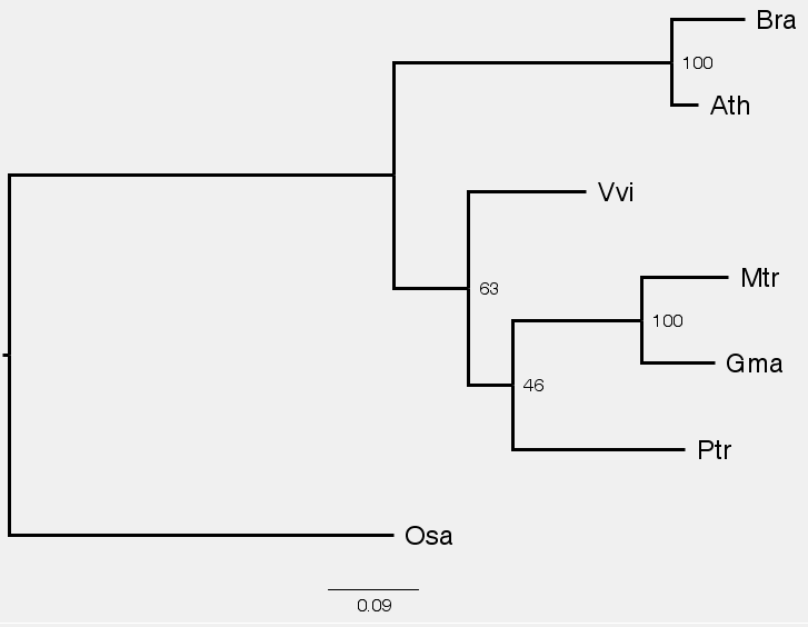
After this step, you would see a tree file "C1.raxml.support", which is a tree file with bootstrapping support values.

less C1.raxml.support

3. Follow the same procedure to do bootstrapping for leafy_align.fas.

raxml-ng  --bootstrap --threads 2 --msa leafy_align.fas --model LG+G4 --prefix B2

raxml-ng  --support --tree A2.raxml.bestTree --bs-trees B2.raxml.bootstraps --prefix C2

less C2.raxml.support

2.4 Using "figtree" to visualize the trees

Use Filezilla to download the two tree files "C1.raxml.support" and "C2.raxml.support" to your laptop. Start "figtree". Open the file "C1.raxml.support". When prompted for names for branches and nodes, enter "BS".

After opening the file in "figtree", check the boxes for "Tip Label" and "Node Label". Expand "Tip Label" and "Node Label" to change "font" and increase size as needed. Expand "Node Label", select "BS" for "Display".

2.5 Combining search and bootstrapping in one command

In practice, we normally use the "--all" function to run raxml-ng, which combines the steps in 2.2 & 2.3 into a single command. The "--all" function is good for small to medium size data set. If you are working with a very large data set, it would be better to run the two steps separately, so that you can customize each step differently.

raxml-ng --all --msa prim.phy --model GTR+G --prefix D1

After this, you would get a tree file with bootstrapping support values: "D1.raxml.support".

2.6 Tree likelihood evaluation

"--evaluate" re-optimizes all branch lengths and model parameters without changing the tree topology. This step is optional, as in most cases, we are more interested in tree topology than the branch lengths.

Evaluate the likelihood of A1.raxml.bestTree under the following models: GTR+G, GTR+R4, GTR, JC and JC+G.

raxml-ng --evaluate --msa prim.phy --tree A1.raxml.bestTree --model GTR+G --prefix E_GTRG

raxml-ng --evaluate --msa prim.phy --tree A1.raxml.bestTree --model GTR+R4 --prefix E_GTRR4

raxml-ng --evaluate --msa prim.phy --tree A1.raxml.bestTree --model GTR --prefix E_GTR

raxml-ng --evaluate --msa prim.phy --tree A1.raxml.bestTree --model JC --prefix E_JC

raxml-ng --evaluate --msa prim.phy --tree A1.raxml.bestTree --model JC+G --prefix E_JCG

ls -lrt

Each "--evaluate" command would create 5 output files, including *.raxml.log, and *.raxml.bestTree.

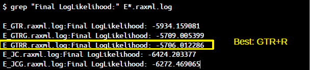
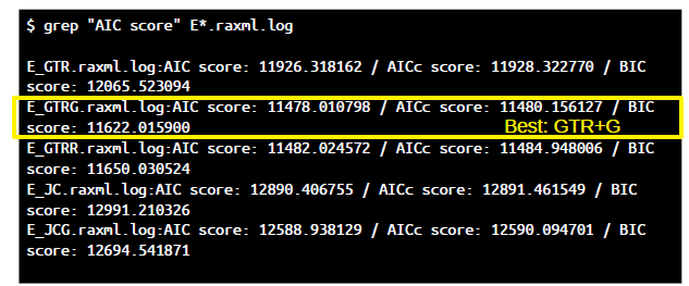
Use "grep" to extract the final likelihood scores from log files produced with the five different models:

grep "Final" E*.raxml.log

grep "AIC score" E*.raxml.log

Which model should be preferred? Compare likelihoods and AIC/AICc/BIC scores (lower=better).

2.7 Using modeltest-ng to find the best model

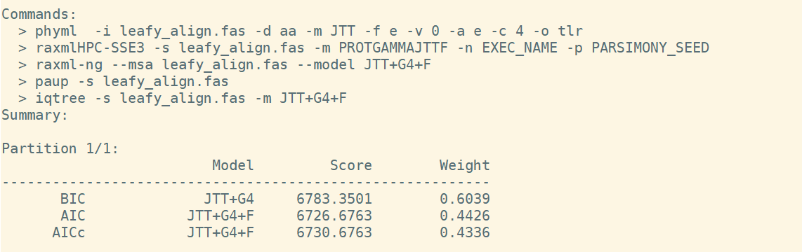
It is always each to determine best model to use. The "modeltest-ng" tool can be used to estimate the best model to use, it also provides you with the actual command to run "raxml-ng search".

/programs/modeltest-0.1.5/modeltest-ng -i leafy_align.fas  -d aa

• When you work on real projects, please check the BioHPC software page (https://biohpc.cornell.edu/lab/userguide.aspx?a=software&i=794#c) to run the latest version. The newer version only works on AVX2 CPUs.

   

Based on the command provided by modeltest-ng output, now you can run raxml-ng as:

raxml-ng --msa leafy_align.fas --model JTT+G4+F --prefix leafy_aa

3. Build NJ tree using vcf file

VCF (https://en.wikipedia.org/wiki/Variant_Call_Format) is a file format commonly used for SNP genotyping results. In this exercise, you will use Tassel to build a Neighbor-Joining tree (NJ) from a VCF file. Tassel ( https://www.maizegenetics.net/tassel) is a very popular genetics software, developed by Ed Buckler lab here at Cornell. You can run Tassel either as a GUI software on your laptop, or as a command-line tool on the server. In this exercise, you will run the command lines on the Linux server.

The parameters:

-Xmx5g: specify the maximum memory size for Java;

-treeSaveDistance false: because we do not supply pre-calculated distance matrix;

-vcf: input vcf file name;

-tree Neighbor: neighbor joining tree;

-exportType Text: output newick format

#export the tree as a human-readable text file
/programs/tassel-5-standalone/run_pipeline.pl -Xmx5g -vcf mdp_genotype.vcf -tree Neighbor -treeSaveDistance false -export tree.nj.txt 

less tree.nj.txt 

#export the tree as a newick file
/programs/tassel-5-standalone/run_pipeline.pl -Xmx5g -vcf mdp_genotype.vcf -tree Neighbor -treeSaveDistance false -export tree.nj.nwk -exportType Text

less tree.nj.nwk

Download the tree file "tree.nj.nwk" to your laptop and open in "figtree". To get the best view, you will need to adjust "Expansion" and "Zoom".

In practice, when you work with VCF files, it is always a good idea to pre-filter the VCF file. (It is the same concept as running "Gblocks" on MSA files, to remove the un-reliable sites). You can use "Tassel", "VCFtools" or "BCFtools" to do the filtering. Commonly used filters including: missing data, allele frequency. You can also use more sophisticated filters like "segregation pattern", "LD", "read depth", et al.

4. Run Orthofinder to identify orthologous genes

Orthofinder is a tool to identify orthologous genes from multiple genomes. In this exercise, you will run the software with sequences from four different E. coli strains. Once you have the ortholog gene groups, you can run MSA software on each ortholog group, followed by Raxml-ng to infer phylogeny.

4.1 Examine and pre-process the input files.

At the beginning of this exercise, you have copied the four E. coli fasta files into your working directory. The files should be under the directory /workdir/$USER/project3/faa, named "*_translated_cds.faa.gz".

Use the command "zcat file_name.gz | head -n 40" to check the first 40 lines of a ".gz" file. Use the command "wc -l" to count the number of genes per strain.

cd /workdir/$USER/project3/faa

ls -l

# check the first 40 lines of the file
zcat GCF_000005845.2_ASM584v2_translated_cds.faa.gz | head -n 40

# count the number of genes in the file
zcat GCF_000005845.2_ASM584v2_translated_cds.faa.gz | grep ">" |wc -l

The protein sequences in the input files have very long titles, like ">lcl|NC_000913.3_prot_NP_414548.1_7 [gene=yaaJ] [locus_tag=b0007] [db_xref=UniProtKB/Swiss-Prot:P30143] [protein=putative transporter YaaJ] [protein_id=NP_414548.1] [location=complement(6529..7959)] [gbkey=CDS]".

There are two potential problems with these sequence titles:

• The titles are too long. Some MSA software cannot work with sequences with long titles;
• Some software would not work with non-alphanumeric characters (except underscore "_");

It would be a good idea to simplify the sequence titles in the fasta files before running Orthofinder. In Linux, the "sed" command can be used to replace text. In the following commands, you will de-compress the original file with "zcat", pipe through two rounds of "sed", and re-direct the output to new files named "strain*.faa".

I also like the sequence titles to start with strain names like "s1" "s2" "s3" "s4", so that in the MSA results, you can easily tell from which strain each sequence comes from. As each input files are different, you will need to use the "sed" command creatively to modify the sequence titles.

• sed "s/ .*//" : In each line, remove everything after the first "space" character.
• sed "s/.*/>s1/": the pattern would replace ">lcl|NC_000913.3_prot_NP_414548.1" with ">s1_".

zcat GCF_000005845.2_ASM584v2_translated_cds.faa.gz | \
   sed "s/ .*//" | \
   sed "s/.*_/>s1_/" \
   > strain1.faa

zcat GCF_003018555.1_ASM301855v1_translated_cds.faa.gz | \
   sed "s/ .*//" | \
   sed "s/.*_/>s2_/" \
   > strain2.faa
   
zcat GCF_003112165.1_ASM311216v1_translated_cds.faa.gz | \
   sed "s/ .*//" | \
   sed "s/.*_/>s3_/" \
   > strain3.faa
   
zcat GCF_006874785.1_ASM687478v1_translated_cds.faa.gz | \
   sed "s/ .*//" | \
   sed "s/.*_/>s4_/" \
   > strain4.faa

After these steps, you will have 4 fasta files with short sequence titles: strain1.faa, strain2.faa, strain3.faa and strain4.faa

Use "grep" to check the sequence titles in the cleaned fasta files:

grep ">" strain1.faa
grep ">" strain2.faa
grep ">" strain3.faa
grep ">" strain4.faa

4.2 Run Orthofinder

Unfortunately, you will not be able to run Orthofinder using the training computers. The software requires CPUs that support AVX2. In BioHPC system, it only works on medium or large memory gen2 computers.

The step-by-step instructions of running Orthofinder on BioHPC can be found on this page: https://biohpc.cornell.edu/lab/userguide.aspx?a=software&i=629#c . It is very straight forward. The software reads in a directory of protein fasta files, and the output is a directory with many files. You will examine the output files in the next step.

4.3 Examine the output files

The output of Orthofinder should be under the working directory /workdir/$USER/project3/. The file is "Results_Oct06.tar.gz".

De-compress the Results_Oct04.tar.gz file:

cd /workdir/$USER/project3/

tar xvfz Results_Oct06.tar.gz

cd Results_Oct06

ls -l

You would find several sub-directories in the Orthofinder results.

First, you will check the files under the directory "Orthogroups".

• Orthogroups.GeneCount.tsv: A tab separated text file. Each row contains the genes belonging to a single ortholog group. The genes from each ortholog group are organized into columns, one per strain.

cd Orthogroups

# check the content of the file
less Orthogroups.GeneCount.tsv

# count the total number of groups
wc -l Orthogroups.GeneCount.tsv

# count the number of groups with one gene per strain
awk '{if (($2==1)&&($3==1)&&($4==1)&&($5==1)) print}' Orthogroups.GeneCount.tsv | wc -l

There is a total of 5411 ortholog groups in the four E. coli strains. Among these groups, 3557 of the groups have one gene per strain, which is ideal for building phylogenetic tree. The ID of these "one-gene-per-strain" ortholog groups are stored in the file "Orthogroups_SingleCopyOrthologues.txt".

• Orthogroups.txt & Orthogroups.tsv: These two files have the names of each gene in the ortholog groups. The two files contain the same information but in different file formats.

less Orthogroups.txt
less Orthogroups.tsv

• Orthogroups_UnassignedGenes.tsv: Singleton genes that were not assigned to any groups

less Orthogroups_UnassignedGenes.tsv

Next let's check the directory Orthogroup_Sequences.

cd /workdir/$USER/project3/Results_Oct06/Orthogroup_Sequences

ls -l

In this directory, you would find 6423 fasta files. Each file contains sequences for an ortholog group. These files can be used to run MSA software.

Last you can check the directory Comparative_Genomics_Statistics, which includes summary reports of the run.

cd /workdir/$USER/project3/Results_Oct06/Comparative_Genomics_Statistics

less Statistics_Overall.tsv

4.4 Run MSA for all single copy genes

Orthofinder output a directory called "Single_Copy_Orthologue_Sequences" which contains fasta files for all single copy genes that are present in every species. These sequences are ideal for construction of a species tree. In this exercise, you will run MSA & Gblocks on each one of the FASTA files.

First you need to create a batch script to process all files in the directory. Linux command "xargs" can be used for this purpose.

cd /workdir/$USER/project3/Results_Oct06/Single_Copy_Orthologue_Sequences

ls *.fa | xargs -I {} echo "mafft --thread 1 --amino  --inputorder --quiet {}  > aln_{} ; Gblocks aln_{} -t=p -b5=h" > msa.batch

less msa.batch

Run the batch script in parallel to take advantage of multiple CPU cores. You will use the "GNU parallel command" to run the batch script, set "-j 2" so that 2 jobs would run simultaneously. This would take a while, run it in "screen".

screen
export PATH=/programs/mafft/bin:$PATH
export PATH=/programs/Gblocks_0.91b:$PATH

parallel -j 2 < msa.batch

After it is done, you should see a set of new files: aln_*.fa-gb. These are the cleaned MSA files.

ls -l *gb

less aln_OG0001399.fa-gb

4.5 Create a species tree from combined MSA of individual ortholog groups

Here you will concatenate all cleaned MSA files into one single fasta file, and create a species tree using raxml-ng .

concate_msa.py: a Python script to concatenate the MSA files of each ortholog groups, and output a single file merged.fasta. (If you will use this script concate_msa.py for your own data, you need to make sure that your files are: 1) In the same order of species, make sure to use " --inputorder" when running mafft or other MSA software to keep the order; 2) Only work with FASTA format.)

mkdir MSAdir

mv *gb MSAdir/

python /shared_data/alignment2020/project3/concate_msa.py MSAdir

raxml-ng --threads 2 --msa merged.fasta --model LG+G4 --prefix merged

The final output is a species tree: merged.raxml.bestTree.